
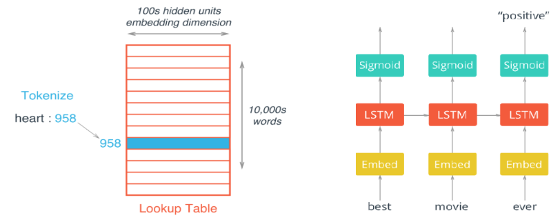
当处理文本中的单词时,传统的one-hot encode会产生仅有一个元素为1,其余均为0的长向量,这对于网络计算是极大地浪费,使用词嵌入技术(Embeddings)可以有效地解决这一问题。Embeddings将单词转化为整数,并且将weight matrix看作一个lookup table(如左图所示),从而避免了稀疏向量与矩阵的直接相乘。
本文首先介绍在RNN中使用Embeddings进行情感分析(sentiment analysis),所使用的网络结构如右图所示;接着介绍一种特殊的词嵌入模型Word2Vec,用来将单词转化成包含语义解释(semantic meaning)的向量。
Sentiment Analysis
使用的数据下载,其中reviews.txt中已将大写字母全部转化为小写字母
- 数据前处理
### 读取数据 with open('sentiment/reviews.txt', 'r') as f: reviews = f.read() #评论 with open('sentiment/labels.txt', 'r') as f: labels = f.read() #情感标签 ### 去掉标点符号 from string import punctuation all_text = ''.join([c for c in reviews if c not in punctuation]) ### 获取评论和单词 reviews = all_text.split('\n') all_text = ' '.join(reviews) words = all_text.split() ### 将单词转化为整数 from collections import Counter counts = Counter(words) vocab = sorted(counts, key=counts.get, reverse=True) #将单词按出现次数从多到少排序 vocab_to_int = {word: ii for ii, word in enumerate(vocab, 1)} #将单词从1开始编码 reviews_ints = [] for each in reviews: reviews_ints.append([vocab_to_int[word] for word in each.split()]) ### 将标签转化为整数 import numpy as np labels = labels.split('\n') labels = np.array([1 if each == 'positive' else 0 for each in labels]) ### 去掉长度为0的评论 non_zero_idx = [ii for ii, review in enumerate(reviews_ints) if len(review) != 0] reviews_ints = [reviews_ints[ii] for ii in non_zero_idx] labels = np.array([labels[ii] for ii in non_zero_idx]) ### 截取评论中的前200个单词,不足200单词的评论在左边补0 seq_len = 200 features = np.zeros((len(reviews_ints), seq_len), dtype=int) for i, row in enumerate(reviews_ints): features[i, -len(row):] = np.array(row)[:seq_len] ### 拆分训练、验证和测试集 split_frac = 0.8 split_idx = int(len(features)*0.8) train_x, val_x = features[:split_idx], features[split_idx:] train_y, val_y = labels[:split_idx], labels[split_idx:] test_idx = int(len(val_x)*0.5) val_x, test_x = val_x[:test_idx], val_x[test_idx:] val_y, test_y = val_y[:test_idx], val_y[test_idx:] - 搭建网络
### 超参数设置 lstm_size = 256 lstm_layers = 1 batch_size = 500 learning_rate = 0.001 embed_size = 300 #Size of the embedding vectors(number of units in the embedding layer) ### Input import tensorflow as tf graph = tf.Graph() #Create the graph object with graph.as_default(): inputs_ = tf.placeholder(tf.int32, [None, None], name='inputs') labels_ = tf.placeholder(tf.int32, [None, None], name='labels') keep_prob = tf.placeholder(tf.float32, name='keep_prob') ### Embed Layer n_words = len(vocab_to_int) + 1 #Adding 1 because we use 0's for padding, dictionary started at 1 with graph.as_default(): embedding = tf.Variable(tf.random_uniform((n_words, embed_size), -1, 1)) embed = tf.nn.embedding_lookup(embedding, inputs_) #3D tensor (batch_size, seq_len, embed_size) ### LSTM Layer with graph.as_default(): lstm = tf.contrib.rnn.BasicLSTMCell(lstm_size) drop = tf.contrib.rnn.DropoutWrapper(lstm, output_keep_prob=keep_prob) cell = tf.contrib.rnn.MultiRNNCell([drop] * lstm_layers) initial_state = cell.zero_state(batch_size, tf.float32) #Getting an initial state ### Output layer with graph.as_default(): outputs, final_state = tf.nn.dynamic_rnn(cell, embed, initial_state=initial_state) logits = tf.contrib.layers.fully_connected(outputs[:, -1], 1, activation_fn=None) #从最后一步的输出(batch_size, lstm_size)建立全连接层 predictions = tf.nn.sigmoid(logits) ### Loss function and Optimizer ### Two options for loss function: ### cost = tf.losses.mean_squared_error(labels_, predictions) ### cost = cross-entropy with graph.as_default(): loss = tf.nn.sigmoid_cross_entropy_with_logits(labels=tf.cast(labels_, tf.float32), logits=logits) cost = tf.reduce_mean(loss) #cross-entropy optimizer = tf.train.AdamOptimizer(learning_rate).minimize(cost) ### Validation and Test Accuracy with graph.as_default(): correct_pred = tf.equal(tf.cast(tf.round(predictions), tf.int32), labels_) accuracy = tf.reduce_mean(tf.cast(correct_pred, tf.float32)) - 训练网络
def get_batches(x, y, batch_size=100): n_batches = len(x)//batch_size x, y = x[:n_batches*batch_size], y[:n_batches*batch_size] for ii in range(0, len(x), batch_size): yield x[ii:ii+batch_size], y[ii:ii+batch_size] ### Train and Validation epochs = 20 best_validation_acc = 0.0 #Best validation accuracy seen so far with graph.as_default(): saver = tf.train.Saver() with tf.Session(graph=graph) as sess: sess.run(tf.global_variables_initializer()) iteration = 1 for e in range(epochs): state = sess.run(initial_state) for x, y in get_batches(train_x, train_y, batch_size): feed = {inputs_: x, labels_: y[:, None], keep_prob: 0.5, initial_state: state} loss, state, _ = sess.run([cost, final_state, optimizer], feed_dict=feed) if iteration%5==0: print("Epoch: {}/{}".format(e, epochs), \ "Iteration: {}".format(iteration), \ "Train loss: {:.3f}".format(loss)) if iteration%25==0: val_acc = [] val_state = sess.run(cell.zero_state(batch_size, tf.float32)) for xv, yv in get_batches(val_x, val_y, batch_size): feed = {inputs_: xv, labels_: yv[:, None], keep_prob: 1, initial_state: val_state} batch_acc, val_state = sess.run([accuracy, final_state], feed_dict=feed) val_acc.append(batch_acc) validation_acc = np.mean(val_acc) print("Val acc: {:.3f}".format(validation_acc)) if validation_acc > best_validation_acc: best_validation_acc = validation_acc #Update the best-known validation accuracy saver.save(sess, "checkpoints/sentiment_best_validation.ckpt") iteration += 1 saver.save(sess, "checkpoints/sentiment_last_iteration.ckpt") - 检验网络
test_acc = []
with tf.Session(graph=graph) as sess:
    saver.restore(sess, 'checkpoints/sentiment_best_validation.ckpt') #should also check sentiment_last_iteration.ckpt
    test_state = sess.run(cell.zero_state(batch_size, tf.float32))
    for xt, yt in get_batches(test_x, test_y, batch_size):
        feed = {inputs_: xt, labels_: yt[:, None], keep_prob: 1, initial_state: test_state}
        batch_acc, test_state = sess.run([accuracy, final_state], feed_dict=feed)
        test_acc.append(batch_acc)
    print("Test accuracy: {:.3f}".format(np.mean(test_acc)))
Word2Vec
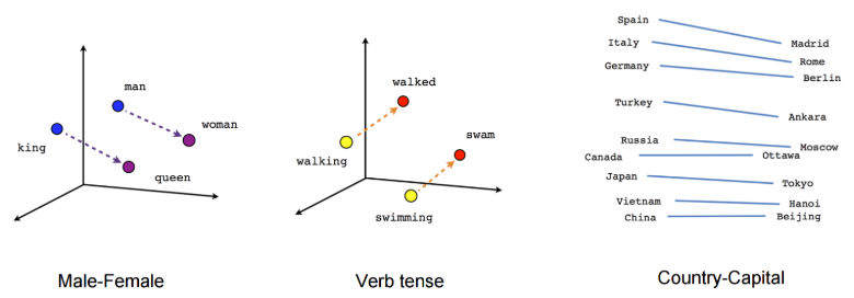
Word2Vec是可以结合上下文语义生成词向量的一种算法,经常在相同语义下出现的词语,它们生成的词向量也很相似(如下图所示),本文所使用的训练数据是Matt Mahoney整理的维基百科文章
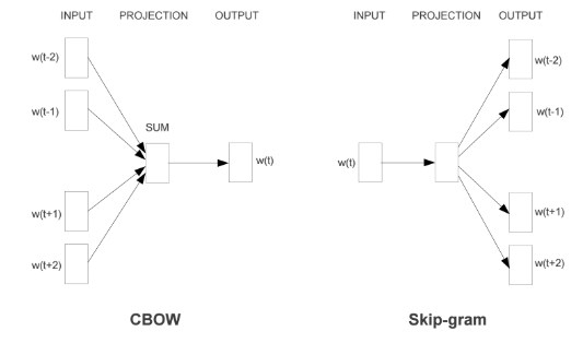
Word2Vec主要有两种架构形式,分别为CBOW(Continuous Bag-Of-Words)和Skip-gram,两种方法的示意图如下图所示。CBOW是用周围词预测中心词,从而利用中心词的预测结果情况,不断地去调整周围词的向量;Skip-gram是用中心词来预测周围的词,利用周围的词的预测结果情况,不断地调整中心词的词向量。
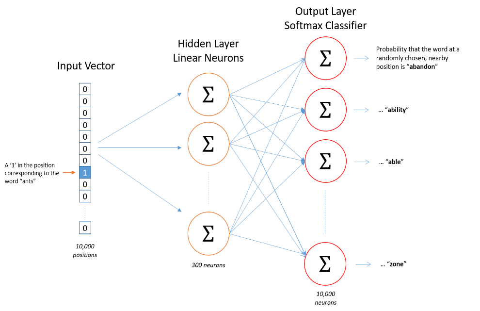
本文主要对Skip-gram进行介绍,采用的网络结构如下图所示。
- 数据前处理
from collections import Counter def process(text): text = text.lower() ### Replace punctuation with tokens so we can use them in our model text = text.replace('.', ' <PERIOD> ') text = text.replace(',', ' <COMMA> ') text = text.replace('"', ' <QUOTATION_MARK> ') text = text.replace(';', ' <SEMICOLON> ') text = text.replace('!', ' <EXCLAMATION_MARK> ') text = text.replace('?', ' <QUESTION_MARK> ') text = text.replace('(', ' <LEFT_PAREN> ') text = text.replace(')', ' <RIGHT_PAREN> ') text = text.replace('--', ' <HYPHENS> ') text = text.replace(':', ' <COLON> ') ### Remove all words with 5 or fewer occurences words = text.split() word_counts = Counter(words) trimmed_words = [word for word in words if word_counts[word] > 5] return trimmed_words ### 读取并处理数据 with open('data/text8') as f: text = f.read() words = process(text) ### 将单词编码为整数 word_counts = Counter(words) sorted_vocab = sorted(word_counts, key=word_counts.get, reverse=True) int_to_vocab = {ii: word for ii, word in enumerate(sorted_vocab)} vocab_to_int = {word: ii for ii, word in int_to_vocab.items()} int_words = [vocab_to_int[word] for word in words] ### Subsampling, 随机去掉一些高频词(例如the) ### for each word in the training data, discard the word with probability 1-sqrt(threshold/word frequency) import random threshold = 1e-5 word_counts = Counter(int_words) total_count = len(int_words) freqs = {word: count/total_count for word, count in word_counts.items()} p_drop = {word: 1 - np.sqrt(threshold/freqs[word]) for word in word_counts} train_words = [word for word in int_words if random.random() < (1 - p_drop[word])] - 获取batch
### 找到所要训练的单词周围的单词 def get_target(words, idx, window_size=5): ### Get a list of words in a window around an index R = np.random.randint(1, window_size+1) start = idx - R if (idx - R) > 0 else 0 stop = idx + R target_words = set(words[start:idx] + words[idx+1:stop+1]) return list(target_words) def get_batches(words, batch_size, window_size=5): ### Create a generator of word batches as a tuple (inputs, targets) ### inputs(or targets) is a list of integers n_batches = len(words)//batch_size words = words[:n_batches*batch_size] #only full batches for idx in range(0, len(words), batch_size): x, y = [], [] batch = words[idx:idx+batch_size] for ii in range(len(batch)): batch_x = batch[ii] batch_y = get_target(batch, ii, window_size) y.extend(batch_y) x.extend([batch_x]*len(batch_y)) yield x, y - 搭建网络,结构如下图所示
import tensorflow as tf train_graph = tf.Graph() ### Input with train_graph.as_default(): inputs = tf.placeholder(tf.int32, [None], name='inputs') labels = tf.placeholder(tf.int32, [None, None], name='labels') ### Embed n_vocab = len(int_to_vocab) n_embedding = 200 #number of embedding features with train_graph.as_default(): embedding = tf.Variable(tf.random_uniform((n_vocab, n_embedding), -1, 1)) embed = tf.nn.embedding_lookup(embedding, inputs) ### Negative Sampling ### The size of our word vocabulary means that our skip-gram neural network has a tremendous number of weights ### All of the weights would be updated slightly by every one of our training samples. This makes training the network very inefficient ### With negative sampling, we are instead going to randomly select just a small number of “negative” words(for which we want the network to output a 0) to update the weights for ### We will also still update the weights for our “positive” word((for which we want the network to output a 1) ### Essentially, the probability for selecting a word as a negative sample is related to its frequency, with more frequent words being more likely to be selected as negative samples n_sampled = 100 #number of negative labels to sample with train_graph.as_default(): ### negative sampling is for training only ### note the shape of softmax_w is (n_vocab, n_embedding) ### if we want to calculate the full softmax loss, use: ### logits = tf.matmul(embed, tf.transpose(softmax_w)) ### logits = tf.nn.bias_add(logits, softmax_b) softmax_w = tf.Variable(tf.truncated_normal((n_vocab, n_embedding), stddev=0.1)) softmax_b = tf.Variable(tf.zeros(n_vocab)) loss = tf.nn.sampled_softmax_loss(softmax_w, softmax_b, labels, embed, n_sampled, n_vocab) #calculate the loss using negative sampling cost = tf.reduce_mean(loss) optimizer = tf.train.AdamOptimizer().minimize(cost) ### Normalize each word's vector with train_graph.as_default(): norm = tf.sqrt(tf.reduce_sum(tf.square(embedding), 1, keep_dims=True)) normalized_embedding = embedding / norm - 训练和验证网络
epochs = 10
batch_size = 1000
window_size = 10
with train_graph.as_default():
    saver = tf.train.Saver()
with tf.Session(graph=train_graph) as sess:
    iteration = 1
    loss = 0
    sess.run(tf.global_variables_initializer())
    for e in range(1, epochs+1):
        batches = get_batches(train_words, batch_size, window_size)
        for x, y in batches:
            feed = {inputs: x, labels: np.array(y)[:, None]} #labels shoud be a 2D tensor (len(y), 1)
            train_loss, _ = sess.run([cost, optimizer], feed_dict=feed)

            loss += train_loss
            if iteration % 100 == 0:
                print("Epoch {}/{}".format(e, epochs), \
                      "Iteration: {}".format(iteration), \
                      "Avg. Training loss: {:.4f}".format(loss/100))
                loss = 0

            iteration += 1
    save_path = saver.save(sess, "checkpoints/text8.ckpt")
    embed_mat = sess.run(normalized_embedding)
### Use T-SNE to visualize word vectors
import matplotlib.pyplot as plt
from sklearn.manifold import TSNE
viz_words = 500
tsne = TSNE()
embed_tsne = tsne.fit_transform(embed_mat[:viz_words, :])
fig, ax = plt.subplots(figsize=(14, 14))
for idx in range(viz_words):
    plt.scatter(*embed_tsne[idx, :], color='steelblue')
    plt.annotate(int_to_vocab[idx], (embed_tsne[idx, 0], embed_tsne[idx, 1]), alpha=0.7)